What is VLOOKUP?
Here’s the definition of VLOOKUP from office.microsoft.com:
Searches for a value in the first column of a table array and returns a value in the same row from another column in the table array. The V in VLOOKUP stands for vertical. Use VLOOKUP instead of HLOOKUP when your comparison values are located in a column to the left of the data that you want to find.
How to use VLOOKUP in Excel
I’ve prepared some example data, which would be considered very typical of the type a digital marketer would find herself using.
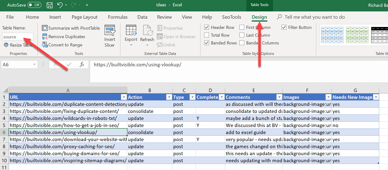
Firstly, we have some raw data in a tab:

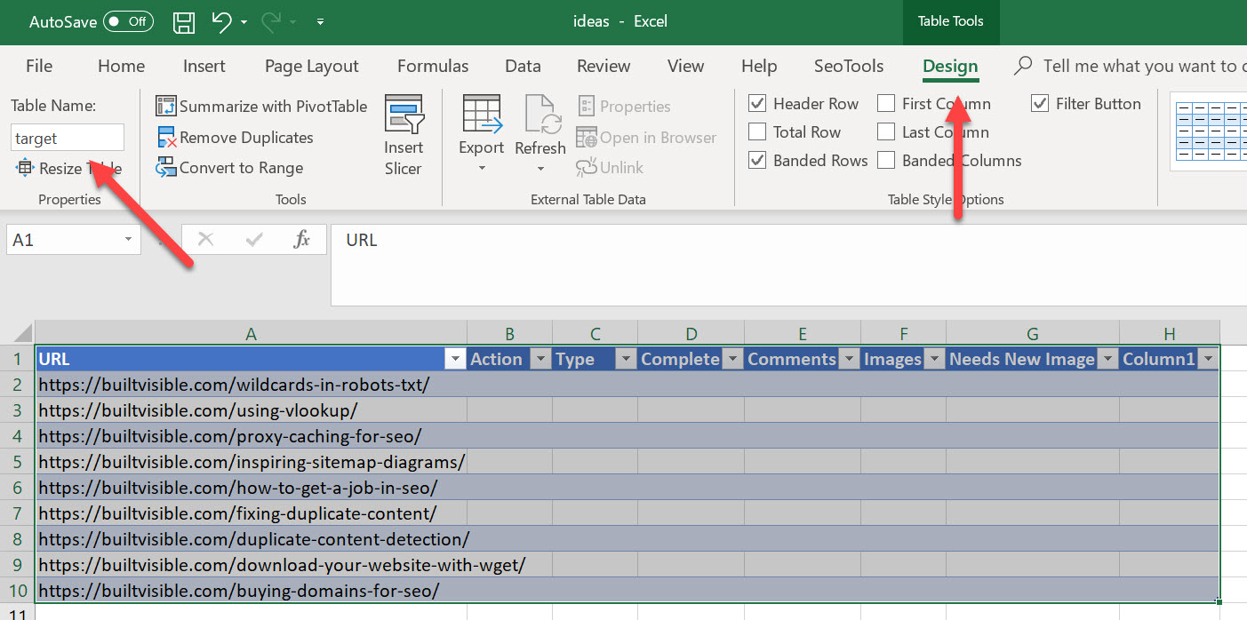
And in another tab, we have a blank collection of data.

I would like to use the “URL” to lookup and fetch data from one table to another. So, first of all, I’m going to create a Table, by clicking in the top cell in the spreadsheet and then using the shortcut: CRTL+SHIFT+down then right to highlight everything in the table, then CTRL+L to create the table.

I’m also going to name my table “source”.

Now I have the data source formatted correctly, I need to repeat the procedure for the target Table. I’ll call that table “target”.

Finally, I can get on with the process of writing the formula.
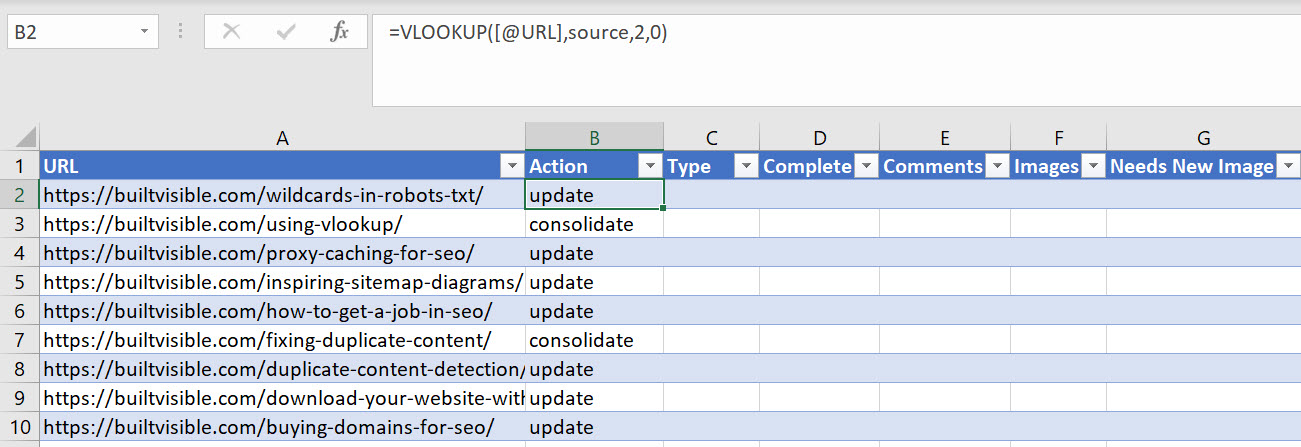
We’re going to look up the 2nd column of the source table and bring that data into our target table, using this formula:
=VLOOKUP([@URL],source,2,0)

Where:
- [@URL] is the URL value in the left most column, and the data used to perfrom the lookup.
- “source” is the name of the table that has the data I need.
- “2” is the column value I wish to return with my formula.
- “0” is EXACT match – either find the exact value and return a result, or return an error.
