VLOOKUP formula
Let’s kick off with one of the most widely used formulas in Excel, VLOOKUP. This formula helps us to quickly search for a value in the first column of a table array and returns a value in the same row from another column in the table array. If you are not familiar with the formula, I highly recommend taking a look at Richard Baxter’s post on VLOOKUP.
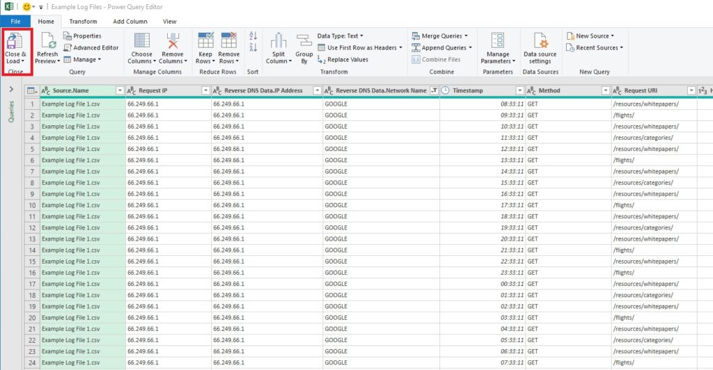
Our goal with using a similar function to in this example will be to filter out requests not made from a verified Google IP. Therefore our focus will be mainly on the “Request IP” column showing what IP address was each request made from.
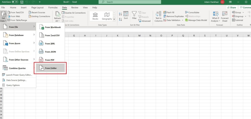
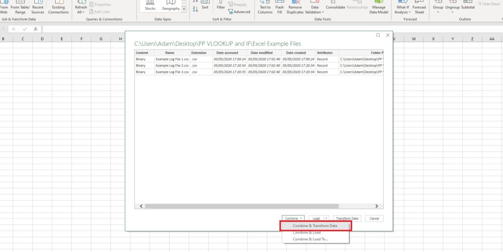
The first thing we will have to do is to get the necessary data loaded into our Power Query Editor. In my example, I will be working with three randomly generated CSV log files each over three million requests.
Click on “Combine & Transform Data” to change and modify the data that we just imported.
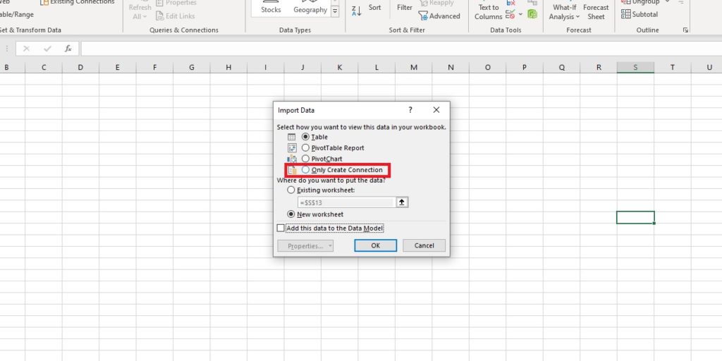
In the Power Query Editor we can format the data as we see fit and these changes will be applied for all three log file datasets. If everything looks as it should, we can proceed with connecting the data by clicking “Close & Load” in the top left corner and “Close & Load To”.
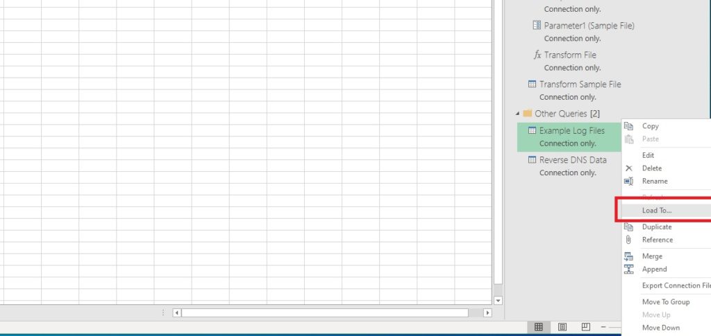
Here we will click on “Only Create Connection” instead of adding it to the Data Model as we did previously. The connection only option will mean there is no data output to the workbook, but you can still use this query in other queries. This will allow us to work with over 1 million rows.
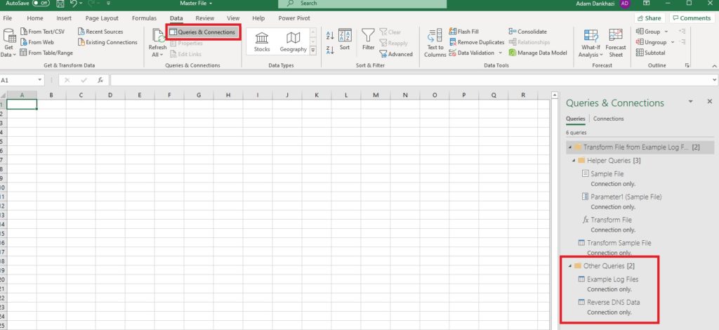
When Excel has finished creating the connection to our query, the “Queries & Connections” sidebar will appear on the right featuring our query under “Other Queries”. If it didn’t appear automatically, you can access it by navigating to the data tab and click on “Queries & Connections”.
In order for us to be able to do our function that’s similar to VLOOKUP, we will also need the reverse DNS data added to our sheet. We can follow the same process to achieve this and when finished, the “Reverse DNS Data” will appear under our Example Log Files within “Other Queries”.
At this point we have all the necessary data for running our function similar to VLOOKUP in the Power Query Editor. To return to the editor, double-click on the Example Log Files within the “Queries & Connections” sidebar.
The function that we will use is called “Merge Queries”.
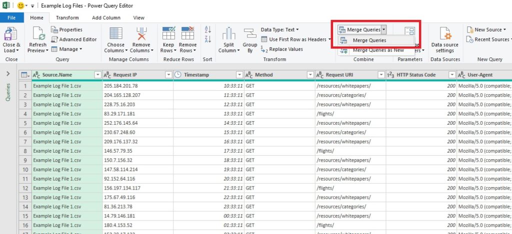
Clicking this button will bring up a new window where we can select which data source we want to use to match information against the IP addresses in our log file.
In this case, we want to get the network name for all request IPs, therefore we will select the “Request IP” column in the log file dataset and the “IP Address” column from the DNS lookup dataset and click “OK”.
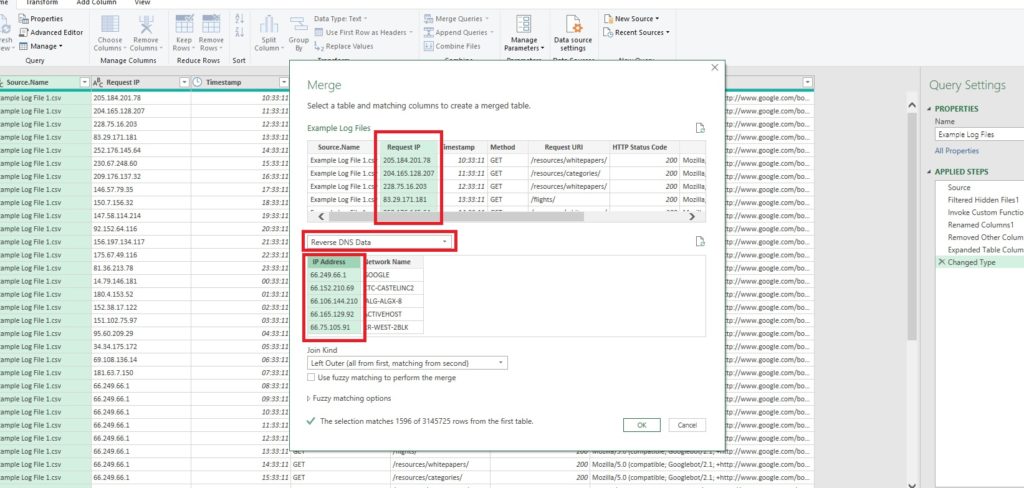
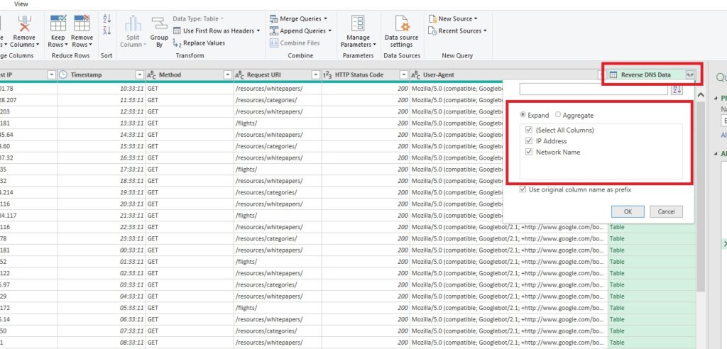
Once the function finishes loading, we can find the data from the reverse DNS lookup sheet in the last column in the Power Query Editor.
This column will contain both the IP address that the function matched up against and the network name. To display the matched data, click on the arrow icon in the header of the new column and select which columns we would like to display.
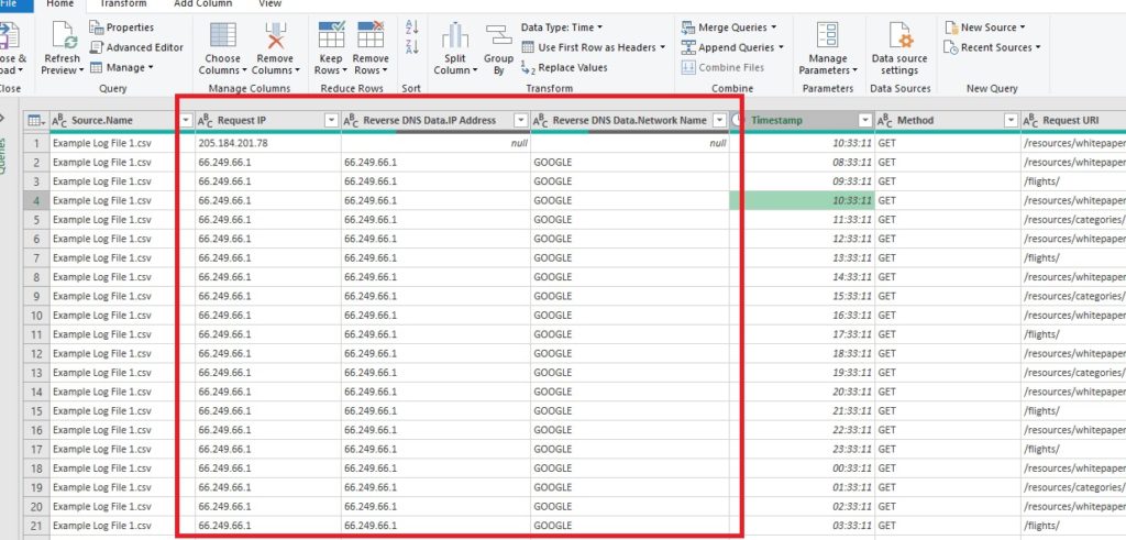
To keep things simple, I’ll move both columns next to the original Request IP column.
As a last step in the editor, we will delete the imported IP address column (Reverse DNS Data IP Address column) and filter all values that aren’t equal to “Google” to get a list of only requests that were made by Google. Click “Close & Save” in the top left corner of the editor to save our query.
To get our filtered list, the last step will be to right-click on the “Example Log Files” query and left-click on “Load to”. Here we will be able to select where we would like to load our data. Select “Load to Table” and our list will be loaded to the active tab.
My example and finalised files can be accessed here for practice: Merge function example files.
IF Formula
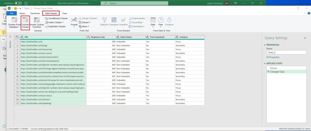
For this formula we will use a Data Analysis Expression (DAX). After moving the data into the Power Query Editor, we will need to create a new “Custom Column” from the “Add Column” tab.
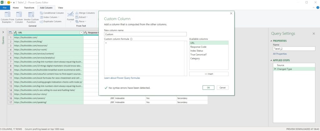
Once this is done, a new window will pop up, where we can set the new column’s name and start writing our IF formula. Even though DAX uses a different syntax to excel formulas, there are also many similarities that will help you to master DAX quickly and easily.
Let’s take a look at an example: I would like to create a new column that tells me if the data within the “index status” column equals “Indexable” or not.
We need to bear in mind a couple of things before writing our formula:
- Formulas in DAX are case sensitive, so make sure you use lowercase characters.
- Instead of using “,” between the logical test values, we use “then” and “else”.
Here is our DAX formula: if [Index Status] = “Indexable” then “yes” else “no”
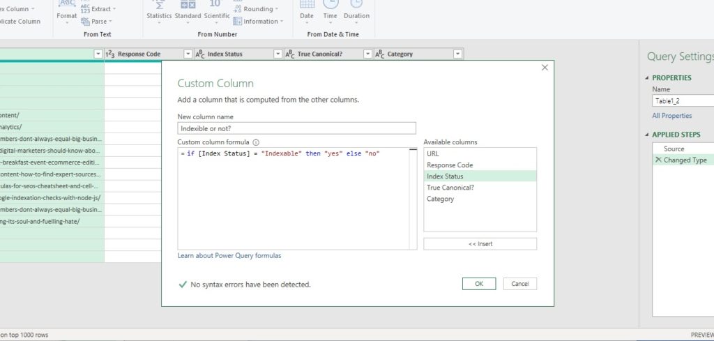
Now, let’s break it down:
Firstly we need to define the type of the formula, which in this case is “if”, followed by the name of the column we want to analyse data in. Then, we’ll need to add in the condition type, which is “=”, and set the condition “Indexable”. Finally, we’ll define what happens when there is a data match with “then” and what happens when there isn’t one with “else”.
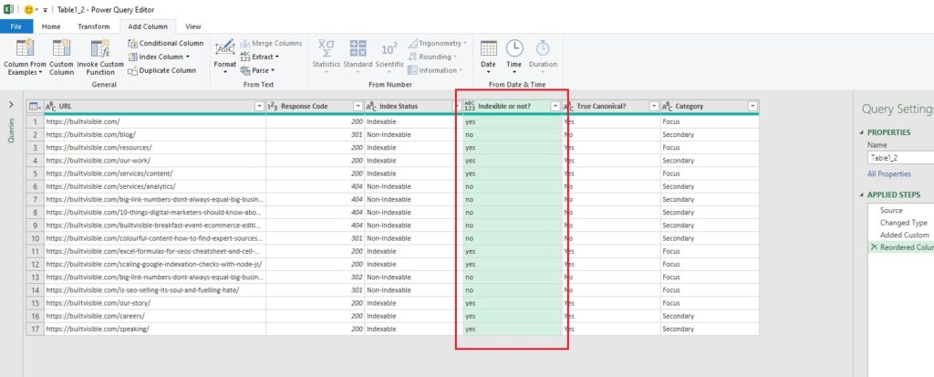
As a result of our formula, a new highlighted column will appear showing which rows match our criteria:
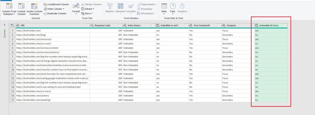
Now, let’s try to create a more advanced formula using multiple criteria. We will create a column that will tell us if our example URL is indexable and also whether it falls into the focus category or not.
This will be our formula:
if [Index Status] = “Indexable” and [Category] = “Focus” then “yes” else “no”
As you can see, it’s very similar to the previous one, but there are a few differences; firstly, we added multiple data columns to be analysed and set a condition for each of them and furthermore, we added “and” to indicate that both criteria have to match in order for the column to return “yes”.
DAX and Power Query functions can be a little intimidating at first, but with a little practice, the basics can be mastered quite easily, opening up entirely new avenues for us when it comes to data processing.
These formulas are quite powerful on their own, but combining them with our Power Query formatting skills can provide a more user-friendly solution to processing large data queries than languages like Python.. In future posts, I will continue to explore how we could bring other popular Excel formulas to life in Power Pivot.
If you have any formula in mind that you would like me to cover, please feel free to leave a comment below.