So, what are these tools exactly?
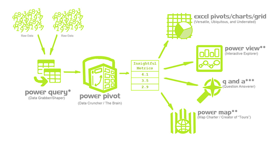
As you can see in the diagram below, Power Query is responsible for merging, organising and cleaning the data you would like to work with. Power Pivot serves as the engine that processes the data and helps you create pivots, charts and grids.
These power tools might look frightening and overly complex at first, but once you learn the basics it’ll be as easy as writing a good formula.
Merging data with Power Query (Get & Transform)
The first step in our journey is importing all the necessary data with Power Query. This tool is absolutely brilliant when it comes to merging, formatting and filtering data.
So where is it located?
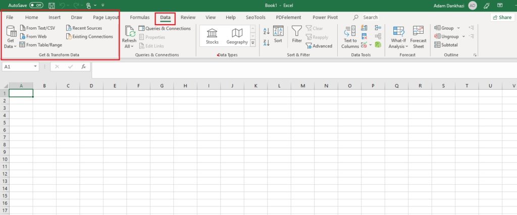
Once you’ve opened Excel, you can find Power Query or “Get & Transform” on the “Data” tab.
As you can see, there‘s a large variety of data sources that you can import from with this tool. For the purpose of this post we’ll stick with importing data from multiple CSV files (as one of the most common types of dataset when it comes to SEO exports) by selecting the folder containing all the TXT/CSV files.
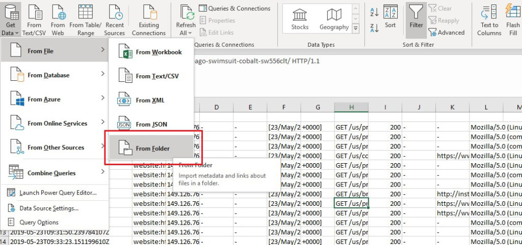
As a first step, I’ll locate the folder that contains the CSV/TXT files that we want to work with and click “OK”.

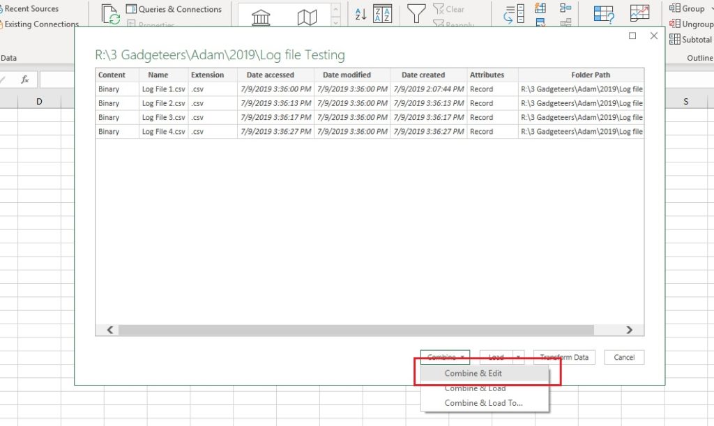
Excel will show us all the files that it has located within the folder. Once happy, we can click “Combine & Edit” to continue, per the image below.
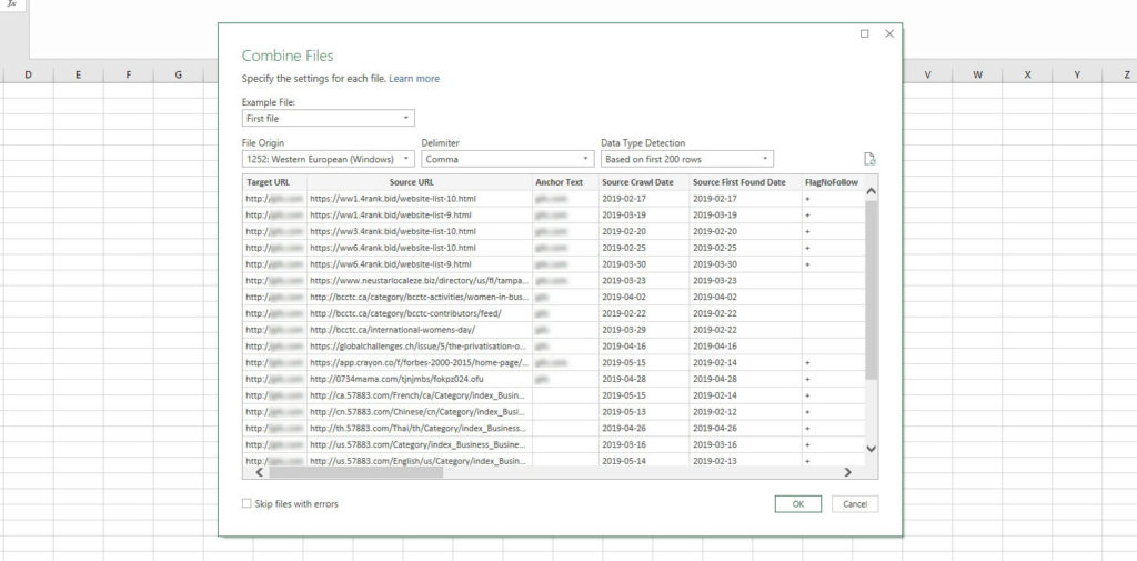
Once all the files have been imported, a sample for each dataset will be available to view, allowing us to ensure that the data is interpreted correctly. If necessary, we can change the delimiter and file encoding. Once done, click OK to enter the Query Editor.
Once this is finished, we can start filtering.
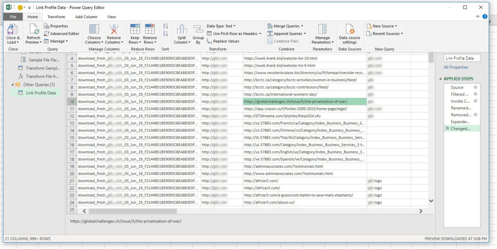
I’m not going to go into too much detail here; most of the functions within the home tab are exactly the same as they are within Excel as standard – removing duplicates, filtering, row insertion, etc. One of the differences is that the filtering in Power Query is much more powerful. It allows us to filter based on more than two criteria for multiple columns at the same time. This can be incredibly useful when you’re analysing large datasets.
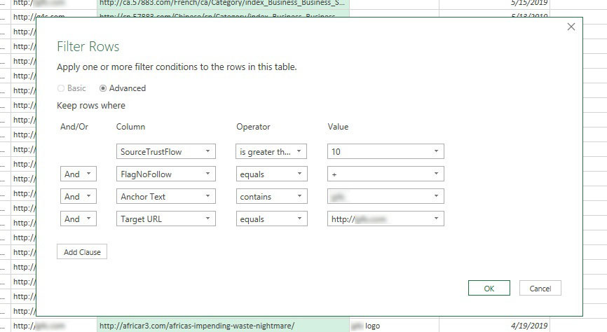
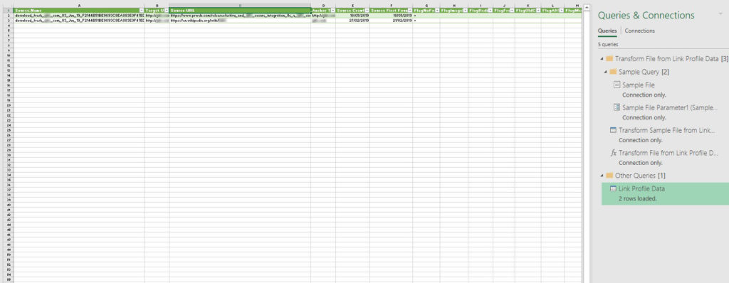
With this filter I’ve instructed Excel to look through nine datasets that were found within the folder “links” (the example data is from Majestic) which have higher TrustFlow than ten, are Nofollow, link to the specific URL and have anchor text containing the brand name.
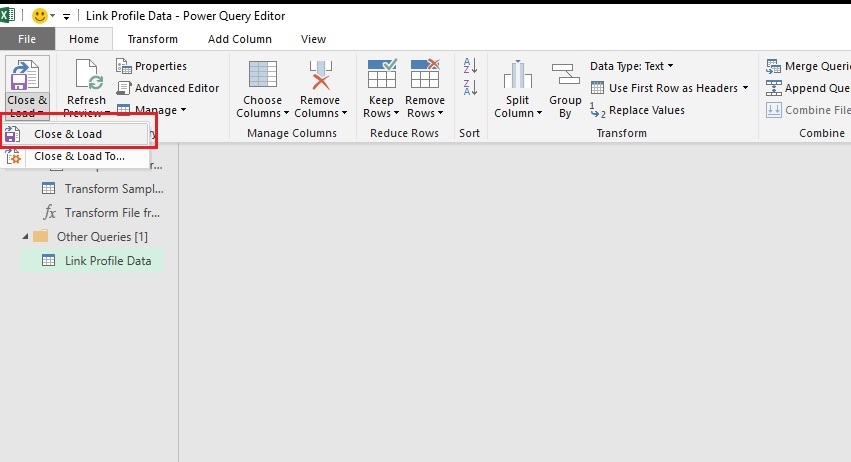
Once you’ve applied the criteria, the editor will filter down the sample dataset in the window. If you see no results don’t be alarmed – the editor only applies your filters to a small portion of the full dataset. To instruct Excel to go through all the data, click on “Close & Load” in the top left corner.
You’ll notice that Excel has created a brand-new tab and a new sidebar has popped up, showing the progress of your data query (on the right side). Once it has finished calculating, all data will be shown from the different data sources filtered down based on your criteria.
One thing to keep in mind is that the maximum row limit (a little over 1 million) also applies here.
Power Pivot
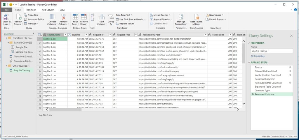
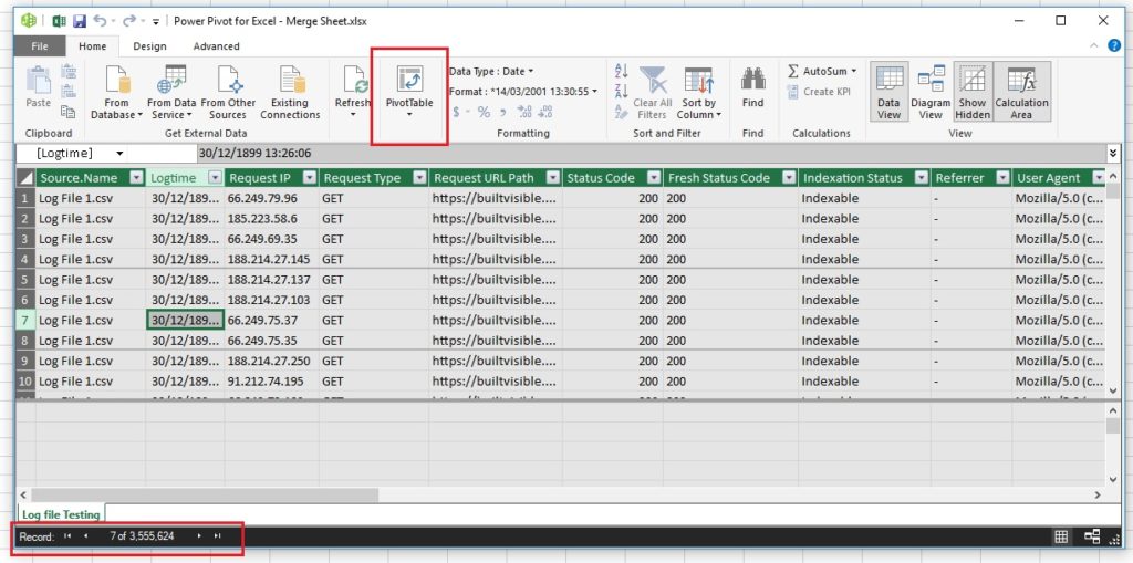
But what if you don’t want to be limited by the 1 million row maximum? You may be surprised to find out that Excel can now manage more than 1 million rows of data. To do so, we will have to add it to the Data Model rather than importing everything into a single tab. This allows Excel to handle and store the imported data more efficiently. I used multiple randomly generated log files for this example containing over 3 million lines.
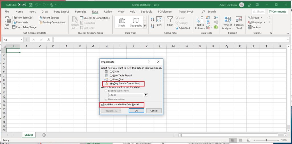
The first thing we will have to do, is to navigate back to the Power Query Editor window and select “Only Create Connection” and “Add this data to the Data Model” instead of importing the data onto a single tab.
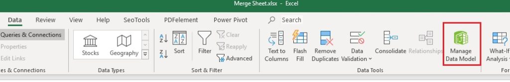
Once the data import has been completed, don’t be alarmed if you don’t see any of data on the sheet. All the data is now stored within Excel’s database, accessed by clicking “Manage Data Model” within the Data or Power Pivot tab.
This will open up the Power Pivot window showing the imported data. As you can see in the bottom left corner, we now have over 3.5 million rows.
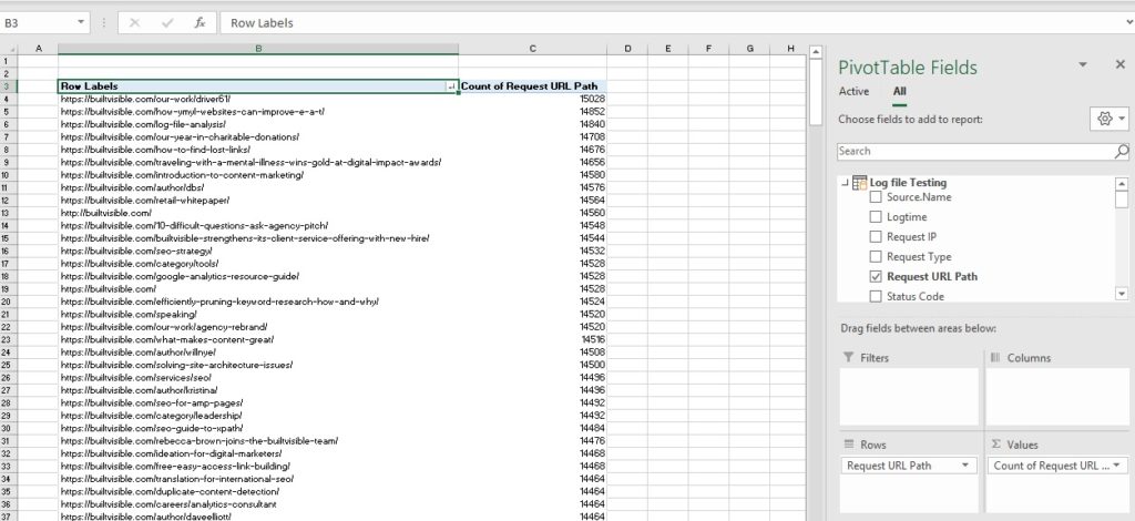
From this point you can immediately start your analysis, using PivotTables to find which pages have been requested the most, the proportion of crawl being wasted, how many requests were made for noindex pages, etc. If you’re looking for a good guide on how to do this, I recommend you give Dan Butler’s guide on Log File Analysis a read.
Taking it a step further
So, this is great: we can now merge multiple sheets together quickly and filter data within them, but how can we add more data to them? How can we add additional crawl data or filter out non-Google requests? In this section I will show how to filter out fake Google requests using Power Pivot and data connections.
We’ll need to do a reverse DNS lookup using a tool such as IPnetInfo or via Python. Once we’ve got the DNS data for all IP addresses listed, we’ll need to add them to a new tab within the Excel sheet that was used to merge.
The next step is to format the data into a table and click on “Add to Data Model” within the Power Pivot tab. This will import you newly added DNS table to the Data Model.
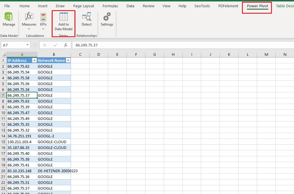
Once done, click on “Manage Data Model” and you will see DNS data on the tab called “Table2”.
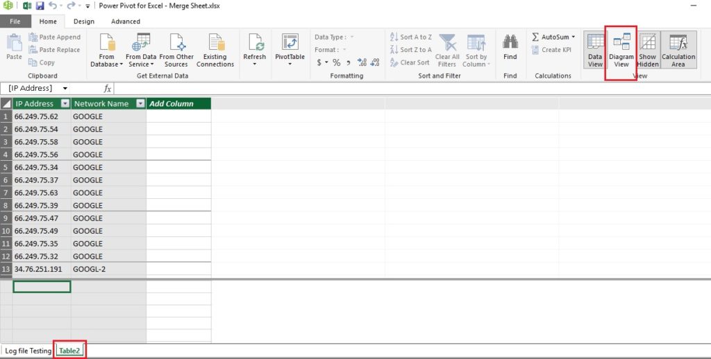
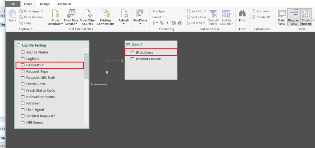
If we were doing this with a smaller dataset, the next step would be to create an additional column that calculates the corresponding network name for all IP addresses. On a dataset of 3.5 million rows this would take a significant amount of time, and most likely result in Excel crashing. What we’ll do instead is create a logical connection between the log files and our newly imported DNS table. This will automatically calculate the network name for each IP.
To do this, bring up the connection view by enabling the “Diagram View” (in the top right corner) and as you can see from my example, I’ve connected the Request IP and the IP Address columns between the two sheets. Once done, create a new pivot table on a new tab.
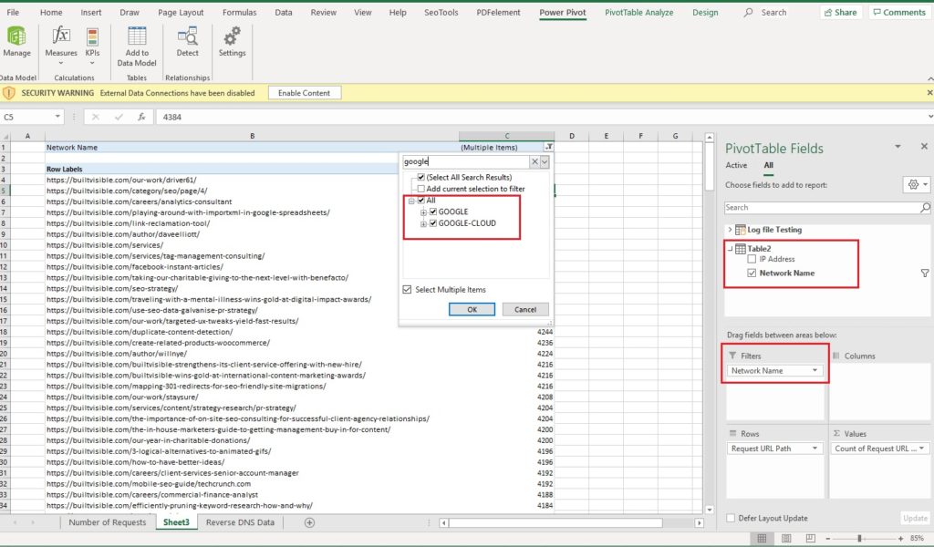
What you can probably spot immediately is that both tables are now accessible in the PivotTable Fields section. Nothing else needs to be done and we can immediately start filtering the data. I’ve filtered out all requests that were not made from the network IDs of Google or Google-Cloud and calculated the total number of requests made for each URL within the datasets.
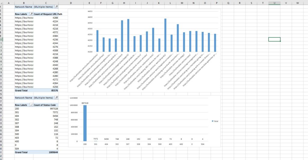
From this point, you can add charts, grids additional pivots and analyse the data in any way you like.
If you’ve followed through my guide you can probably already tell that we’ve barely scratched the surface of what these tools can do. In future articles I’ll be further exploring Power Query and Power Pivot functions using DAX (Data Analysis Expressions).

Colby
Question: does this only work on a Windows OS at the moment? If not, is there an alternative method for importing the add-ins on a Mac?
I’m on a 365 and made sure I’m up-to-date on my Mac, but don’t have the Files > Option > etc function. Looked into Office Add-ins, but couldn’t find it there.
Any help you can provide would be much appreciated!
Adam Dankhazi
Hi Colby,
Sadly the Power BI tools such as Power Query and Power Pivot are available for Windows only and as far as I’m aware there are no plans to make it Mac compatible. What you can try to do is use Bootcamp or Parrallels to run a Windows OS on your Mac. Or something else I’ve heard about is turbo.net that runs excel for you in the cloud, I haven’t tried this yet but sounds interesting. Hope this helps, if you have any questions let me know.
Thanks,
Adam
Faisal Anderson
“It allows us to filter based on more than two criteria for multiple columns at the same time” You have literally saved me years off my life in excel thank you!
Adam Dankhazi
Hi Faisal,
I’m really glad that it helped you! I know it was a huge help for me too :)
Thanks,
Adam